
Basic Structure of My Evidential Arguments
Epistemic Interpretation of Probability
In this article series, when I refer to probability I shall be adopting the epistemic interpretation of probability. The epistemic probability of a statement is a measure of the probability that a statement is true, given some stock of knowledge. In other words, epistemic probability measures a person’s degree of belief in a statement, given some body of evidence. The epistemic probability of a statement can vary from person to person and from time to time (based upon what knowledge a given person had at a given time).[1] For example, the epistemic personal probability that a factory worker Joe will get a pay raise might be different for Joe than it is for Joe’s supervisor, due to differences in their knowledge.
Two Types of Evidence and Corresponding Probabilities
Let us divide the evidence relevant to naturalism and theism into two categories. First, certain items of evidence function as “odd” facts that need to be explained. Second, other items of evidence are background evidence, which determine the prior probability of rival theories and partially determine their explanatory power.
These two types of evidence have two probabilistic counterparts which are useful for evaluating explanatory hypotheses: (1) the prior probability and (2) the explanatory power of a hypothesis H. (1) is a measure of how likely H is to occur based on background information B alone, whether or not E is true. As for (2), this measures the ability of a hypothesis (combined with background evidence B) to predict (i.e., make probable) an item of evidence.[2]
Notation
Let us proceed, then, to defining some basic probabilistic notation.
B: background evidence
E: the evidence to be explained
H: an explanatory hypothesis
Ri: the rival explanatory hypotheses to H
Pr(x): the probability of x
Pr(x | y): the probability of x conditional upon y
Next, let us define the following conditional probabilities.
Pr(H | B) = the prior probability of H with respect to B—a measure of how likely His to occur at all, whether or not E is true.
Pr(Ri | B) = the prior probability of Riwith respect to B—a measure of how likely Ri is to occur at all, whether or not E is true.
Pr(E | H & B) = the explanatory power of H—a measure of the degree to which the hypothesis Hpredicts the data E given B.
Pr(E | Ri & B) = the explanatory power of Ri—a measure of the degree to which Ri predicts E given B.
Pr(H | E& B) = the final probability that His true conditional upon the total evidence Band E.
Bayes’s Theorem
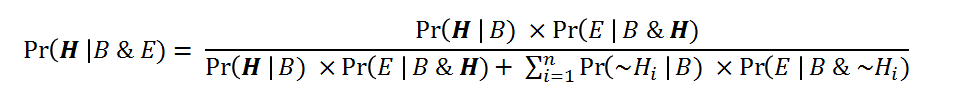
Bayes’s Theorem is a mathematical formula which can be used to represent the effect of new information upon our degree of belief in a hypothesis. In its general form, Bayes’s Theorem may be expressed as follows:
Explanatory Arguments
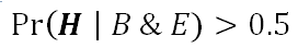
It follows from Bayes’s Theorem that H will have a high final epistemic probability on the evidence B and E:
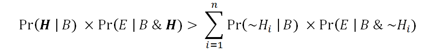
just in case it has a greater overall balance of prior probability and explanatory power than do its alternatives collectively:
Using this insight enables us to easily define the following argument schema for the explanatory arguments in this series.
Let F be some fact and H1 and H2 be rival explanatory hypotheses.
1. F is known to be true, i.e., Pr(F) is close to 1.
2. H1 is not intrinsically much more probable than H2, i.e., Pr(H1 | B) is not much more probable than Pr(H2 | B).
3. Pr(F | H2) > Pr(F | H1).
4. Other evidence held equal, H1 is probably false, i.e., Pr(H1 | B& F) < 0.5.[3]
Evaluating Auxiliary Hypotheses
It is often be useful to determine the evidential significance of an auxiliary hypothesis. In the course of considering various explanatory arguments for naturalism and against theism, we will consider several auxiliary hypotheses. Here are four examples.
- The Evidential Argument from Scale: compares naturalism to theism conjoined with various auxiliary hypotheses about God’s potential reasons for giving or not giving humans a privileged position in the universe.
- The Evidential Argument from the Flourishing and Languishing of Sentient Beings: compares naturalism conjoined with Darwnism to theism conjoined with Darwinism
- The Evidential Argument from the Self-Centeredness and Limited Altruism of Human Beings: compares naturalism conjoined with Darwnism to theism conjoined with Darwinism
- The (Evidential) Fine-Tuning Argument: compares theism to naturalism conjoined with the multiverse hypothesis
In the explanatory argument schema described above, it may be possible to defeat premise (3) by showing that an auxiliary hypothesis is evidentially significant in the relevant way, i.e., that A sufficiently raises Pr(F | H1) or lowers Pr(F | H2). In order to assess the evidential significance of such hypotheses, we would need to apply the theorem of the probability calculus known as the theorem of total probability.
If we let A represent some auxiliary hypothesis, then it follows from the theorem of total probability that:
Pr(F | H1) = Pr(A | H1) x Pr(F | A& H1) + Pr(~A | H1) x Pr(F | H1& ~A)
In the context of explanatory arguments, Draper calls that theorem the “weighted average principle” (WAP).[4] As Draper points out, this formula is an average because Pr(A | H1) + Pr(~A | H1) = 1. It is not a simple straight average, however, since those two values may not equal 1/2; that is why it is a weighted average.[5] The higher Pr(A | H1), the closer Pr(F | H1) will be to Pr(F | A& H1); similarly, the higher Pr(~A | H1), the closer Pr(F | H1) will be to Pr(F | H1& ~A).[6]
Cumulative Cases
Suppose that F is partitioned into 3 facts, F1, F2, and F3,such that F is logically equivalent to F1 & F2& F3. One could easily formulate three independent explanatory arguments for H1 over H2, by showing that each item of evidence individually is antecedently more probable on H1 than on H2, i.e., Pr(F1| H1) > Pr(F1 | H2), Pr(F2 | H1) > Pr(F2 | H2), and Pr(F3 | H1) > Pr(F3| H2). But how could one show that the items of evidence collectively are antecedently more probable on H1 than on H2? In other words, how could one give a about cumulative case argument?
Using the chain rule, it is possible to give a formal, mathematical definition for a cumulative case argument. Using the chain rule it follows that :
Pr(F | H & B) = Pr(F1 & F2 & F3 | H & B)= Pr(F1| H & B) x Pr(F2| F1 & H & B) x Pr(F3 | F1& F2 & H & B)
Therefore, F1, F2, and F3are a cumulative case for H1 and against H2 just in case:
Pr(F | H1 & B) = Pr(F1 & F2 & F3 | H1 & B)= Pr(F1| H1 & B) x Pr(F2| F1 & H1 & B) x Pr(F3 | F1& F2 & H1 & B)
is greater than:
Pr(F | H2 & B) = Pr(F1 & F2 & F3 | H2 & B)= Pr(F1| H2 & B) x Pr(F2| F1 & H2 & B) x Pr(F3 | F1& F2 & H2 & B)Another way to compare these two values is to compare the ratio of H1’s final probability to H2’s final probability. The ratio of these two formulas gives us Bayes’s Theorem in its compound odds form:

If this ratio is greater than 1, then H1’s final probability is greater than H2’s final probability; if the ratio is less than 1, then vice versa; if the ratio equals one, then H1 and H2 have equal final probabilities.This insight gives us one way to show that one hypothesis has a higher final probability than the other hypothesis. For example, suppose want to show that H2 has a higher final probability than H1. In other words, we want to show that:

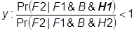
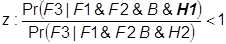
One way to show that H2 has a higher final probability than H1 is to show that the ratio of each multiplicand on the right-hand side of Bayes’s Theorem in its compound odds form is also less than 1, i.e.,
and

and
and
This enables us to define the following schema for cumulative case arguments.
1. Pr(F1 | H2 & B) > Pr(F1 | H1 & B). [from formula x]
2. Pr(F2 | F1& H2 & B) > Pr(F2 | F1& H1 & B). [from formula y]
3. Pr(F3 | F1& F2 & H2 & B) > Pr(F3 | F1 & F2& H1 & B). [from formula z]
4. Some fact F is known to be true, i.e., Pr(F | B) is close to 1.
5. H2 is intrinsically more probable than H1, i.e., Pr(H2 | B) > Pr(H1 | B). [from formula w]
6. Other evidence held equal, H1 is probably false, i.e., Pr(H1 | B& E) < 0.5. [By Bayes’s Theorem]
This schema can obviously be expanded as needed to incorporate the desired number of cumulative lines of evidence.
Notes
[1] Brian Skyrms, Choice & Chance: An Introduction to Inductive Logic (4th ed., Belmont: Wadsworth, 2000), 23.
[2] I owe these definitions to Robert Greg Cavin in private correspondence.
[3] I owe this schema to Paul Draper.
[4] Paul Draper, “Pain and Pleasure: An Evidential Problem for Theists” Noús 23 (1989): 331-50 at 340.
[5] Draper 1989.
[6] Draper 1989.